


Grade 11 statistics lesson
Normal Probability Distribution: Formula, Chart, and Examples
A normal probability distribution is a bell-shaped continuous distribution described by its mean and standard deviation.
Is this already covered?
Not as a full lesson. The site has probability tools that mention the normal, or Gaussian, distribution, and the Z-Score Calculator helps with standardizing values.
This page gives the normal probability distribution its own explanation, formulas, chart, and worked examples.
The normal distribution is different from a binomial distribution because it is continuous. Instead of adding bars for exact values, we find area under a smooth curve.
Normal probability distribution definition
A normal probability distribution is a continuous probability distribution with a symmetric bell shape.
Most values are near the center, and values become less common as they move farther away from the mean.
If \(X\) follows a normal distribution with mean \(\mu\) and standard deviation \(\sigma\), we write:
\[X\sim N(\mu,\sigma^2)\]
The mean \(\mu\) controls the center. The standard deviation \(\sigma\) controls the spread.
Normal distribution formula
The probability density function for a normal distribution is:
\[f(x)=\frac{1}{\sigma\sqrt{2\pi}}e^{-\frac{(x-\mu)^2}{2\sigma^2}}\]
This formula gives density, not an exact probability at one point.
For a continuous distribution, \(P(X=x)=0\). Probability comes from the area under the curve over an interval.
Normal probability distribution chart
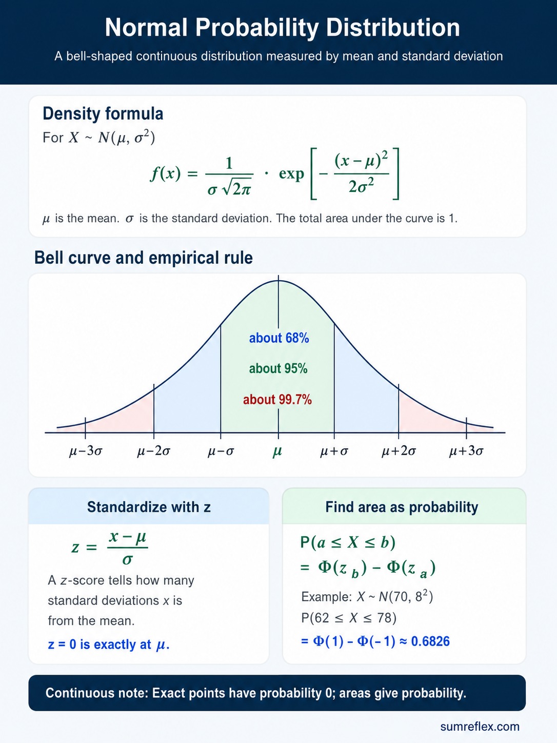
Use this chart to connect the bell curve, the density formula, z-score standardization, and interval probability.
The chart also shows the empirical rule: about 68% of values are within 1 standard deviation, about 95% are within 2, and about 99.7% are within 3.
What the mean and standard deviation do
The mean \(\mu\) is the balance point of the normal curve. It is also the median and the mode for a normal distribution.
The standard deviation \(\sigma\) tells how spread out the curve is.
A small \(\sigma\) makes the curve narrow and tall. A large \(\sigma\) makes the curve wider and flatter.
The total area under every normal curve is always 1, because total probability is 1.
Standard normal distribution
The standard normal distribution is the normal distribution with mean 0 and standard deviation 1.
It is written as:
\[Z\sim N(0,1)\]
Standard normal tables and many calculators use \(Z\) values to find areas under the curve.
Z-score formula
To use the standard normal distribution, convert a raw value \(x\) into a z-score.
\[z=\frac{x-\mu}{\sigma}\]
A z-score tells how many standard deviations a value is from the mean.
If \(z=0\), the value is exactly at the mean. If \(z=2\), the value is 2 standard deviations above the mean. If \(z=-1\), the value is 1 standard deviation below the mean.
Example 1: find a z-score
Suppose test scores are normally distributed with mean 70 and standard deviation 8. Find the z-score for a score of 86.
Step 1: Identify the values: \(\mu=70\), \(\sigma=8\), and \(x=86\).
Step 2: Substitute into the z-score formula: \[z=\frac{86-70}{8}\]
Step 3: Simplify: \[z=\frac{16}{8}=2\]
Answer: A score of 86 is 2 standard deviations above the mean.
Area and probability
In a normal distribution, interval probability is area under the curve.
For a value between \(a\) and \(b\), standardize both endpoints and subtract standard normal CDF values:
\[P(a\le X\le b)=\Phi\left(\frac{b-\mu}{\sigma}\right)-\Phi\left(\frac{a-\mu}{\sigma}\right)\]
The symbol \(\Phi(z)\) means the standard normal cumulative distribution function. For a slower review of cumulative probability, use the cumulative distribution function lesson.
Example 2: probability between two values
Suppose \(X\sim N(70,8^2)\). Find \(P(62\le X\le78)\).
Step 1: Standardize the lower endpoint: \[z_a=\frac{62-70}{8}=-1\]
Step 2: Standardize the upper endpoint: \[z_b=\frac{78-70}{8}=1\]
Step 3: Use the standard normal CDF: \[P(62\le X\le78)=\Phi(1)-\Phi(-1)\]
Step 4: Use common table values: \[\Phi(1)\approx0.8413,\quad \Phi(-1)\approx0.1587\]
Step 5: Subtract: \[0.8413-0.1587=0.6826\]
Answer: The probability is about \(0.6826\), or \(68.26\%\).
Empirical rule
The empirical rule is a quick estimate for normal distributions.
About \(68\%\) of values are within 1 standard deviation of the mean: \[\mu-\sigma\le X\le\mu+\sigma\]
About \(95\%\) of values are within 2 standard deviations of the mean: \[\mu-2\sigma\le X\le\mu+2\sigma\]
About \(99.7\%\) of values are within 3 standard deviations of the mean: \[\mu-3\sigma\le X\le\mu+3\sigma\]
Example 3: use the empirical rule
A machine fills bags with mean weight 500 g and standard deviation 12 g. Assume the weights are approximately normal.
Estimate the percent of bags between 488 g and 512 g.
Step 1: Notice that \(488=500-12\) and \(512=500+12\).
Step 2: The interval is \(\mu-\sigma\) to \(\mu+\sigma\).
Step 3: Use the empirical rule: about \(68\%\) of values lie within 1 standard deviation.
Answer: About 68% of bags are expected to weigh between 488 g and 512 g.
Normal CDF
The normal CDF gives the area to the left of a value.
For a normal random variable \(X\), this is:
\[F(x)=P(X\le x)\]
For the standard normal variable \(Z\), the CDF is written as \(\Phi(z)\).
Because the normal curve is continuous, \(P(X\le x)\) and \(P(X\lt x)\) have the same value.
Normal approximation to binomial
A normal distribution can sometimes approximate a binomial distribution when the number of trials is large and the probability is not too close to 0 or 1.
For \(X\sim\operatorname{Binomial}(n,p)\), the matching normal model uses:
\[\mu=np,\qquad \sigma=\sqrt{np(1-p)}\]
A continuity correction is often used when converting a discrete binomial question into a continuous normal area.
The exact binomial formula is still the better choice for small \(n\) or highly unbalanced probabilities.
For count data based on an average event rate, see the Poisson distribution lesson.
Calculator connection
For quick area checks, use the Probability Calculator and choose the Normal / Gaussian distribution option.
For standardizing raw values or converting between probabilities and z-scores, use the Z-Score Calculator.
Use the calculator after you identify the mean, standard deviation, and whether the question asks for left-tail, right-tail, or between-values probability.
When a normal model is reasonable
A normal model is most reasonable when the data are roughly symmetric, single-peaked, and not heavily affected by extreme outliers.
Measurements such as heights, manufacturing variation, and test scores are often modeled with a normal curve when the situation supports it.
A normal model is not a good automatic choice for counts that cannot go below 0, strongly skewed data, or data with a hard boundary near the center of interest.
Common mistakes
Do not treat the height of the curve as the probability. Probability is area under the curve.
Do not forget to standardize with \(z=(x-\mu)/\sigma\) before using standard normal values.
Do not use the empirical rule for a distribution unless it is normal or approximately normal.
Do not write \(P(X=x)\) as a positive number for a continuous normal distribution. Exact-point probability is 0.
Do not confuse \(\sigma\) with \(\sigma^2\). The notation \(N(\mu,\sigma^2)\) uses variance as the second parameter.
Quick practice
1. If \(X\sim N(50,5^2)\), what are the mean and standard deviation? Answer: mean \(50\), standard deviation \(5\).
2. If \(\mu=40\), \(\sigma=4\), and \(x=48\), what is the z-score? Answer: \(z=(48-40)/4=2\).
3. In a continuous normal distribution, what is \(P(X=70)\)? Answer: 0.
4. About what percent of values lie between \(\mu-2\sigma\) and \(\mu+2\sigma\) in a normal distribution? Answer: about 95%.