Conditional Probability Distribution - Formula and Examples

Does the CDF lesson cover this?

Not fully. A cumulative distribution function answers questions such as \(P(X\le x)\), so it adds probability up to a cutoff value.

A conditional probability distribution answers a different question: what does the whole distribution look like after a condition is known?

For example, a CDF might tell the chance that a commute time is 30 minutes or less. A conditional distribution might tell the commute-time probabilities after we already know it is raining.

Conditional probability distribution definition

A conditional probability distribution is the probability distribution of one random variable after another event or random variable value has been given.

For discrete random variables, the main formula is:

\[P(X=x\mid Y=y)=\frac{P(X=x\text{ and }Y=y)}{P(Y=y)}\]

This formula only works when \(P(Y=y)>0\). If the condition has zero probability, the ratio is not defined in this basic discrete form.

Conditional probability distribution chart

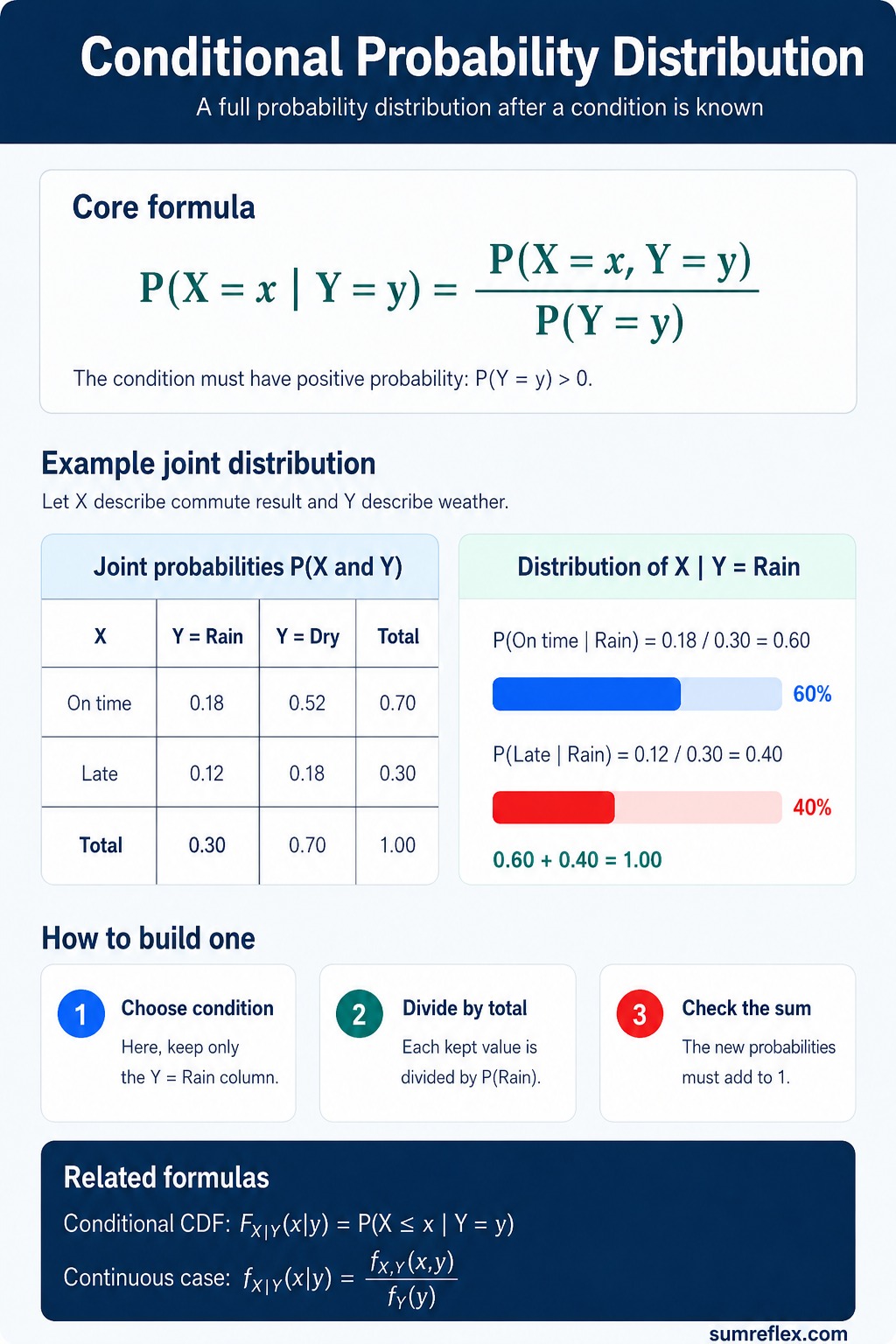
The chart shows how a joint probability table turns into a conditional distribution.

First keep the values that match the condition. Then divide those values by the probability of the condition. The new probabilities should add to 1.

What the condition does

A condition acts like a filter. It says: only look at the part of the probability model where the condition is true.

After filtering, the remaining probabilities usually do not add to 1 yet. Dividing by the condition probability rescales them into a new distribution.

That is why conditional distributions are still real probability distributions. Every probability is between 0 and 1, and all the listed probabilities add to 1.

Discrete example from a joint table

Suppose \(X\) describes whether a commute is on time or late, and \(Y\) describes whether the weather is rain or dry.

The joint probabilities are:

\[P(X=\text{on time},Y=\text{rain})=0.18,\quad P(X=\text{late},Y=\text{rain})=0.12\]

The total probability of rain is:

\[P(Y=\text{rain})=0.18+0.12=0.30\]

Find the conditional distribution of \(X\) given that \(Y=\text{rain}\).

Step 1: Use the conditional distribution formula: \[P(X=x\mid Y=\text{rain})=\frac{P(X=x\text{ and }Y=\text{rain})}{P(Y=\text{rain})}\]

Step 2: Find the on-time probability: \[P(X=\text{on time}\mid Y=\text{rain})=\frac{0.18}{0.30}=0.60\]

Step 3: Find the late probability: \[P(X=\text{late}\mid Y=\text{rain})=\frac{0.12}{0.30}=0.40\]

Answer: Given rain, the conditional distribution of \(X\) is 0.60 on time and 0.40 late.

Check that it is a distribution

A conditional distribution must add to 1 across all possible values of the variable being described.

In the commute example:

\[0.60+0.40=1.00\]

That check matters. If the conditional probabilities do not add to 1, either a value was missed or the denominator was chosen incorrectly.

Conditional probability vs conditional distribution

A conditional probability is one probability after a condition is known.

Example: \(P(X=\text{late}\mid Y=\text{rain})=0.40\).

A conditional distribution gives all the probabilities for the variable after the condition is known.

Example: \(P(X=\text{on time}\mid Y=\text{rain})=0.60\) and \(P(X=\text{late}\mid Y=\text{rain})=0.40\).

Marginal, joint, and conditional distributions

A joint distribution describes two variables together, such as \(P(X=x\text{ and }Y=y)\). The joint probability lesson explains the table and overlap idea in more detail.

A marginal distribution describes one variable by itself, such as \(P(Y=y)\). It is often found by adding across a row or column.

A conditional distribution describes one variable after another value is known, such as \(P(X=x\mid Y=y)\).

The connection is: \[P(X=x\mid Y=y)=\frac{\text{joint probability}}{\text{marginal probability of the condition}}\]

Reverse conditioning changes the question

The statement \(P(X=x\mid Y=y)\) is not the same as \(P(Y=y\mid X=x)\). Reversing the condition usually changes the denominator.

Using the same table, suppose we want the probability of rain given that the commute is on time.

The total probability of an on-time commute is \(0.18+0.52=0.70\).

\[P(Y=\text{rain}\mid X=\text{on time})=\frac{0.18}{0.70}\approx0.257\]

So the probability is about 25.7%, not 60%. The 60% answer belonged to a different condition: on time given rain.

Conditional CDF

A conditional distribution can also have a conditional cumulative distribution function.

The notation is:

\[F_{X\mid Y}(x\mid y)=P(X\le x\mid Y=y)\]

This means: after \(Y=y\) is known, add the probabilities for \(X\) up to \(x\).

So a conditional CDF combines two ideas: the filtering idea from conditional probability and the accumulating idea from a CDF.

Continuous conditional distribution

For continuous random variables, probabilities are described with density functions instead of single exact probabilities.

If \(X\) and \(Y\) have joint density \(f_{X,Y}(x,y)\), then the conditional density of \(X\) given \(Y=y\) is:

\[f_{X\mid Y}(x\mid y)=\frac{f_{X,Y}(x,y)}{f_Y(y)}\]

This formula works where \(f_Y(y)>0\). The conditional density must integrate to 1:

\[\int_{-\infty}^{\infty} f_{X\mid Y}(x\mid y)\,dx=1\]

Independence check

If two variables are independent, knowing one variable does not change the distribution of the other.

For discrete variables, independence gives:

\[P(X=x\mid Y=y)=P(X=x)\]

If the conditional distribution is different from the original distribution of \(X\), then \(X\) and \(Y\) are not independent.

Bayes formula connection

Conditional distributions are closely connected to Bayes formula because Bayes formula reverses the condition.

For discrete values:

\[P(Y=y\mid X=x)=\frac{P(X=x\mid Y=y)P(Y=y)}{P(X=x)}\]

This is useful when one conditional probability is easier to model than the reverse conditional probability.

Common mistakes

Do not divide by the total sample space after a condition is given. Divide by the probability of the condition.

Do not swap \(P(X=x\mid Y=y)\) and \(P(Y=y\mid X=x)\). They usually answer different questions.

Do not call one conditional probability a full distribution unless every possible value has been listed.

Do not forget to check that the conditional probabilities add to 1.

Quick practice

1. If \(P(X=1\text{ and }Y=2)=0.15\) and \(P(Y=2)=0.50\), what is \(P(X=1\mid Y=2)\)? Answer: \(0.15/0.50=0.30\).

2. If \(P(X=0\mid Y=5)=0.25\), \(P(X=1\mid Y=5)=0.35\), and \(P(X=2\mid Y=5)=0.40\), is this a valid conditional distribution? Answer: yes, because \(0.25+0.35+0.40=1\).

3. If \(P(X=x\mid Y=y)=P(X=x)\) for every value of \(x\), what does that suggest? Answer: knowing \(Y=y\) does not change the distribution of \(X\).

4. In a table, why do we divide by the column total when conditioning on a column? Answer: the column total is the probability of the condition.